Jackson Spargur

This project began in my Math Modeling class in my fourth year of college, at a time when I was becoming less interested in baseball statistics, and more interested in bringing some of the innovations of baseball statistics to ultimate frisbee analysis. They are two wildly different sports to analyze: baseball is all about the batter pitcher interaction, and the quantifiable outcomes of that interaction (out, single, double, home run, etc.). Ultimate frisbee really only has two outcomes, those being goals scored for or against. What happens in between is nebulous - passes between players in every direction, sometimes gaining and sometimes losing ground, until eventually a pass can find its way into the hands of a player in their opponent’s endzone. Keeping the disc from being turned over to the other team is in one sense the main objective, but in times of desperation throwing it as far as possible downfield, with no hope of completing a pass can be the right move for the sake of field position alone. Those familiar with football will understand this concept, but other parts, like the fact that there is no one quarterback (though there are “handlers”, which are similar), and that any player can pass the disc any direction at any time invites parallels instead with sports like soccer, and basketball as well. As this is a relatively niche sport, I’ll introduce Ultimate briefly below.

Ultimate Frisbee, or Ultimate is a sport played between two teams of 7 players, on a field measuring 40 yards wide and 70 yards long, plus two 25-yard endzones. Before each point, each team lines up on the endzone lines, and the team on defense throws a “pull”, or kickoff to the other team by throwing it as far downfield as possible. The offensive team must then pass the disc back up the field, attempting to score a goal by catching the disc in the defense’s endzone. Players cannot run with the disc, they can only pivot on one leg - similar to basketball - while it is in their possession. All other players can move freely, and the disc moves when it is thrown to one of these freely moving players (who, upon catching the disc, must then stop and pivot until they find a receiver). One defender, the “mark” in this case, will stand no closer than a disc width from the player with the disc, trying to screen them from throwing an effective pass and also counting loudly and slowly to ten. The rest of the defenders will either shadow an offensive player to prevent them from getting open, or rove around, attempting to intercept passes from their intended receivers. If a pass does not reach its receiver, either because it finds the ground first, or it is dropped, or it is caught but out of bounds, or it is caught or hit to the ground by a defender, or if the thrower fails to release the disc before the mark has counted to ten - the disc is turned over, and the defense takes possession of the disc and attemps to score in the other endzone.

Players are divided into “handlers” and “cutters”, though how many of each there are and how important is the distinction between the two roles depends on the team and the offensive strategy. In general, handlers will run the offense by passing the disc amongst themselves, trying to gain the best field position to throw to open cutters - while cutters will make “cuts” up and down the field in an attempt to get open, passing the disc back to a waiting handler if they do receive the disc but don’t see another open downfield cutter immediately. Players may also be divided into “O-line” or “D-line” players. Players can be substituted with no limitations between points, and larger teams will often have seven offensive specialists (the O Line) to take the points where their team starts on offense, and seven defensive specialists (the D Line) to take the points where the team starts on defense. Of course, each of these “lines” needs to have handlers, cutters, and proficient defenders, but for example, a player with great handling skills but slightly subpar defense would likely wind up the O-line handler, as if all goes well, they won’t need to play defense.

Luckily for my analysis project, I had access to plenty of players. I was on my school’s team, and I was recovering from a nasty hamstring strain which left me with not much to do at tournaments but function as the designated stat-keeper - which for this semester alone was just fine by me. My goal for the project was an individual player statistic based on a predictive model, a model to project the likelihood of scoring a goal that a given player could contribute on any point to their team. This, of course, would be based on their past performance in a number of variables which would have to be shown as being correlated in a significant way to the likelihood of goal scoring. I began trying to use binary logistic regression to pair variables such as Ds (defensive blocks), unforced offensive errors (throwaways, drops, or being stalled - henceforth in total “errors”), and the flight time of players’ pulls to the probability that a goal would be scored. This approach showed some immediate promise: errors were very well (negatively) correlated with scoring probability on O points, and Ds were very well (positively) correlated with goal scoring on D points. And these regressions, being logistic, even modeled

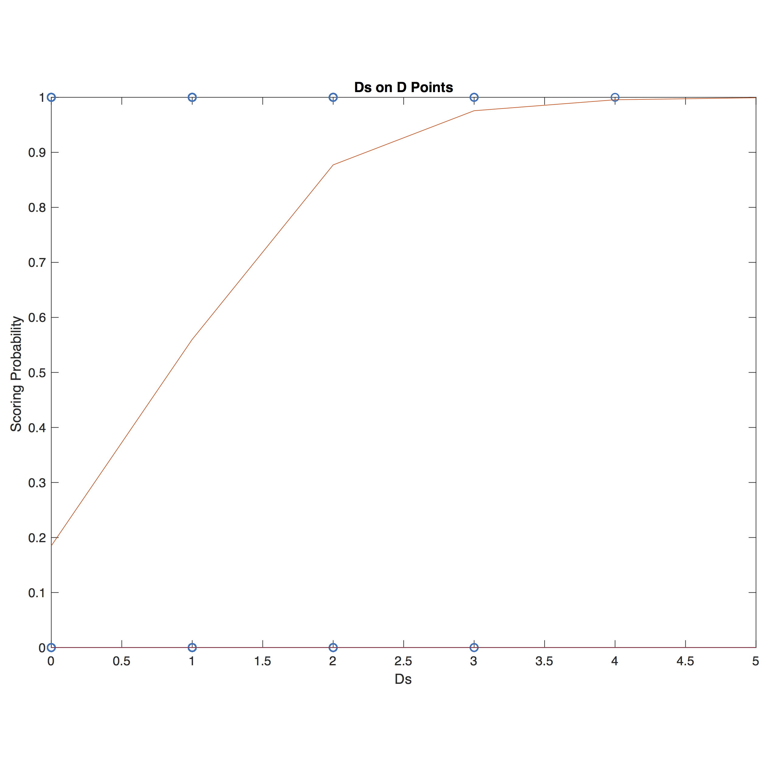
Figure 1: Binary logistic regression for scoring probability vs number of Ds on defensive points

defensive turnovers in a point. The two variables go hand in hand. A player can accrue, for example, a large amount of offensive turnovers, and a small amount of defensive turnovers over the course of a few games, but the premise of a multivariate regression with errors and Ds would be something like: “what’s the probability of scoring on a point where the defense made x Ds, and the offense turned it over y times?” Say we wanted to plug in the statistics of a player who had accrued 40 Ds and 10 errors - we would be asking the question: “what’s the probability of scoring on a point where the defense got 40 Ds but the offense turned it over 10 times?” It’s an impossible premise. My method soon proved to be a bit too simplistic, and while this is usually a good way to err when building a model, in this case, I had simply underestimated the problem.

I tried a few other approaches, but never really landed on one that made much sense in terms of the mechanics of the game. I presented my work at the end of the semester as an unanswered question, and let the data sit in a folder for a few years as I moved onto other classes and other projects.

A few years and two undergraduate degrees later I was thinking about graphs - as in the data structure - when it occurred to me that it could be a perfect way to represent an Ultimate dataset. In a graph every data point is a “node”, and nodes can be connected with “edges” - which themselves can carry information. It’s a very powerful and intuitive data structure, and one particularly well-suited to a dataset where the most important features of the data are the connections between the data points. In this case, the nodes would represent individual play events, and the edges would connect the nodes in the order they occurred. Graphs can be “directed” or “undirected”, and I would use a directed graph so that edges would only point “one way”, and represent an order of events from the beginning to the end of each point. If duplicate strings of events occurred, I would not make a new branch for each occurrence, but note down the number of times each node was visited and branch as necessary. Each string of events would begin at the same two places: with either a goal for or a goal against (signifying either a defensive point or an offensive point), and they would each end with one of those two results as well. The end result of this would be two trees, one for offensive points and one for defensive points, between them containing each and every unique point of Ultimate played in the dataset.

What would be the point of this, other than making some more cool figures? I was still thinking about that probabilistic model from my senior year, and how to make use of this data organization method to answer the question I had asked so long ago. The beauty of the graph representation is that it provides a great solution. Each point concludes with a goal, either for or against. The implication of this is that every position on the graph has a certain probability of leading to a goal for a particular team. All I would need to do is travel to every leaf of the tree reachable from a given node (remember, this is using a directed graph, so nodes are only reachable in the forward direction), calculate how many times each leaf had been visited, and which leaves represented goals for rather than against. If I calculated this probability for every node in the graph, I could know the impact of every

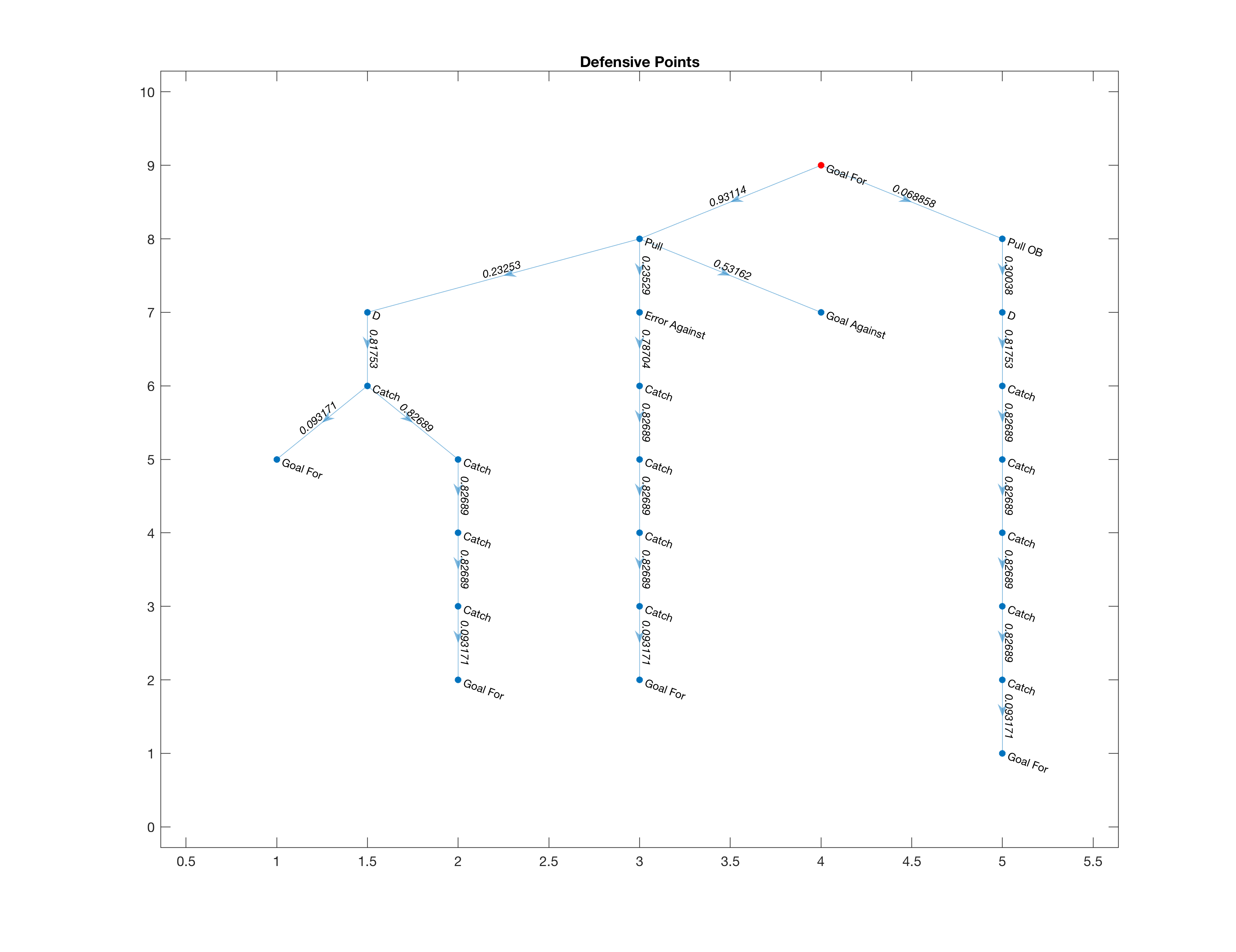
Figure 2: Graph visualization of five defensive points in my dataset. Note how the potential for analysis lies at the junctures between nodes, where a player could either lead their team down a branch less likely to lead to a goal, or more likely. The numbers on the edges represent the context-free transition probabilities between events - for example in any situation a catch (completed pass) was 83% likely to lead to another completed pass in my data

running through every play that every player was involved in, and calculating the effect that each of these plays had on scoring probability, I would be able to keep a tally, for every player, of the cumulative probability that they have added or subtracted over the course of their playing time in the dataset.

Every point is not created equal in Ultimate, however, and I wanted to know how many goals each of these players added or subtracted. A player may accumulate 100% scoring probability, but teams don’t start points with a 0% chance of scoring - especially when they start on offense. Ultimate, especially high-level Ultimate, heavily favors the offense.

Typically the offensive team starts the point with about a 70% probability of scoring, and the defense likewise with a 30% probability of scoring. Therefore, for a player to contribute a “goal” on a point which they started on the offensive team, they must accrue 30% probability, whereas a player starting on defense needs to build up 70%. This may seem like an unfair penalty towards primarily D-line players, but just like every point isn’t created equally, all probability is not created equally. Imagine a situation where an O-line player and a D-line player both manage to singlehandedly score a goal. Say, the O-line player catches the pull, puts a deep shot up, an opposing defender tips it in the air (meaning the player can now legally catch their own throw), and the player does catch their own throw - all the way in the other team’s endzone for a goal. Now imagine a D-line player pulls the disc to the other team, and then immediately callahans (intercepts an opponents throw in their own endzone leading to an immediate goal). They both carried their lines singlehandedly to a goal, but what the D-line player did was much easier. The first player had to sprint the entire length of the field, and was only by chance even legally allowed to make the goal-scoring catch. However, because this O-line player’s team was already favored to score 7 times out of 10, all their heroics didn’t add all that much, whereas the D-line player’s far easier play added an entire 70% to their team’s scoring probability. Their rewards in terms of raw probability skew far towards the D-line player, but when taking into account the base scoring probability of offensive and defensive points, both players are awarded the same: 1 Total Goal.

I wanted a bigger set of data to work with for this, as a greater number of plays on record would mean greater accuracy with regards to the scoring probability of each node. I downloaded the entire 2018 AUDL (a semi-pro Ultimate league, home to most of the best talent in Ultimate right now) season from Ultianalytics, a site which allows Ultimate scorekeepers to keep track of every play. I chose the AUDL because club teams, which also offer an elite level of play but following a more traditional rule set (the AUDL changes a few things, but nothing too fundamental), do not keep stats as scrupulously as the teams in the AUDL do. Before I present a leaderboard, I think it is probably worth a disclaimer that while I started this project at the very beginning with the aim to create a predictive model of performance, Total Goals is not that. Players who perform well in this statistic are most likely good players, and thus are probably going to continue to be good, but my approach here was different from the approach of regression statistics, wherein one finds a model that fits the data and uses it as an indicator of what can be expected of the player given certain variable inputs. What I’ve created here is just one way to look at what already happened. We know that a certain number of goals were scored, and how. The question Total Goals attempts to answer is who contributed the most to those goals, in a probabilistic sense?

Disclaimer out of the way, here are three tables, representing the top 20 players in Total Goals, Total Offensive Goals, and Total Defensive Goals. The latter two don’t refer to goals on the O line or D line, but to goals added from offensive play/defensive play, regardless of how the points began.

I think I’m relatively happy with this effort, and I think in terms of significance and utility it at least serves as a more numerically meaningful version of the popular +/- statistic, a basic shorthand holistic value statistic which awards players for events like goals and assists and docks them for mistakes, like drops or throwaways. Total Goals does the same, but assigns a meaningful value to those events.

While this process in total is a little computationally taxing, I would love to see a system where plays were put in a graph as games commenced, constantly adding to the graph until almost every possible sequence of plays imaginable was represented. That would allow something like the win probability bar chess engines employ, or the one Fangraphs hosts at their site for MLB games. Both of these sports have an incredible amount of past data from which to calculate win probability, and I think using my approach to catalogue play sequences would be one way to bring that to Ultimate.

Of course, the future of Ultimate analysis is in metrics based on accurate field position readings. Colloquially in Ultimate we speak of gaining “power position” - essentially moving the disc near the sideline where there is more open airspace to throw to a cutter on a deep route - and I’m sure a careful analysis of scoring tendencies based on field position could reveal optimizations to offensive and defensive strategy nobody has begun to imagine. Until Ultimate is played in radar-equipped facilities a-la baseball, however, that may have to wait.